Let's examine our data sources to understand the challenge at hand. We're working with two Excel sheets containing similar data, but they're structured differently—a common scenario in enterprise data management:
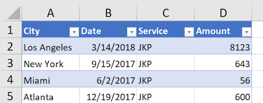
Source 1:
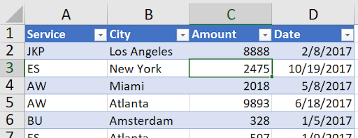
(This dataset extends through row 123, representing a substantial collection of records.)
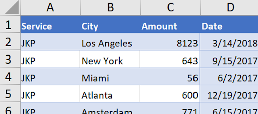
Source 2:
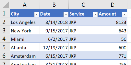
(This dataset continues to row 127, containing overlapping but differently organized information.)
The key challenge becomes immediately apparent: the column structures don't align. Notice how the City field appears in column B in Source 1 but shifts to column A in Source 2. This misalignment is typical when working with data from different departments, systems, or time periods. The question becomes: how do we elegantly combine this disparate data using a single formula to achieve a unified result like this:
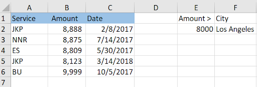
What makes this solution particularly powerful is its dynamic nature. Row 2 in our results draws from Source 1, while row 5 pulls from Source 2—all seamlessly integrated. The real magic happens when we modify our filter criteria. When the city parameter in cell F2 changes, watch what happens:
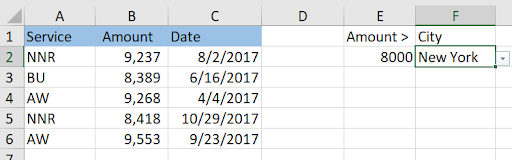
The results instantly update, drawing relevant records from both sources. Similarly, adjusting the amount threshold in cell E2 triggers a complete refresh of the filtered data. This level of responsiveness transforms static spreadsheets into dynamic analytical tools.
Now let's dissect the sophisticated formula powering this functionality—all contained within a single cell (A2).
The Complete Formula:
=IFERROR(CHOOSECOLS(LET(All, VSTACK(Source1!A2:D,000, CHOOSECOLS(Source2!A2:D,000,3,1,4,2)), FILTER(All, (INDEX(All,,3)>E2)*(INDEX(All,,2)=F2))),1,3,4), "None")
This formula represents modern Excel at its most powerful, leveraging advanced functions introduced in Excel 365. Let's break it down systematically, starting from the inside out.
Step 1: Column Restructuring with CHOOSECOLS
We'll begin by examining this highlighted section:
=IFERROR(CHOOSECOLS(LET(All, VSTACK(Source1!A2:D,000, CHOOSECOLS(Source2!A2:D,000,3,1,4,2)), FILTER(All, (INDEX(All,,3)>E2)*(INDEX(All,,2)=F2))),1,3,4), "None")
The CHOOSECOLS function serves as our data harmonization tool. The range Source2!A2:D,000 captures all data rows (excluding headers) with extra capacity for future growth—a best practice for dynamic ranges. The sequence "3,1,4,2" performs the crucial column reordering. Here's the transformation in action:
Original Source 2 structure:
Reordered to match Source 1:
This column resequencing ensures both datasets follow identical structures before integration.
Step 2: Data Consolidation with VSTACK
With our columns aligned, we can now stack the datasets vertically:
=IFERROR(CHOOSECOLS(LET(All, VSTACK(Source1!A2:D,000, CHOOSECOLS(Source2!A2:D,000,3,1,4,2)), FILTER(All, (INDEX(All,,3)>E2)*(INDEX(All,,2)=F2))),1,3,4), "None")
VSTACK performs the vertical concatenation entirely in memory—no temporary worksheets required. This approach maintains formula efficiency and reduces file complexity.
Step 3: Variable Assignment with LET
=IFERROR(CHOOSECOLS(LET(All, VSTACK(Source1!A2:D,000, CHOOSECOLS(Source2!A2:D,000,3,1,4,2)), FILTER(All, (INDEX(All,,3)>E2)*(INDEX(All,,2)=F2))),1,3,4), "None")
The LET function, one of Excel's most significant recent additions, allows us to store our consolidated dataset in a variable named "All." This eliminates redundant calculations and makes our formula more readable—critical when building complex analytical models that others need to maintain.
Step 4: Intelligent Filtering
=IFERROR(CHOOSECOLS(LET(All, VSTACK(Source1!A2:D,000, CHOOSECOLS(Source2!A2:D,000,3,1,4,2)), FILTER(All, (INDEX(All,,3)>E2)*(INDEX(All,,2)=F2))),1,3,4), "None")
Our FILTER function applies two simultaneous conditions: amounts must exceed the threshold in E2, and cities must match the value in F2. The multiplication operator (*) creates an AND condition—both criteria must be satisfied. For OR conditions, you would use addition (+) instead. The INDEX functions reference specific columns: INDEX(All,,3) targets the amount column, while INDEX(All,,2) focuses on the city column.
Step 5: Output Optimization
=IFERROR(CHOOSECOLS(LET(All, VSTACK(Source1!A2:D,000, CHOOSECOLS(Source2!A2:D,000,3,1,4,2)), FILTER(All, (INDEX(All,,3)>E2)*(INDEX(All,,2)=F2))),1,3,4), "None")
The outer CHOOSECOLS statement refines our output by excluding the city column (column 2) from results. Since all filtered results share the same city, displaying it would be redundant. The "1,3,4" selection presents only the essential information.
Step 6: Error Handling
=IFERROR(CHOOSECOLS(LET(All, VSTACK(Source1!A2:D,000, CHOOSECOLS(Source2!A2:D,000,3,1,4,2)), FILTER(All, (INDEX(All,,3)>E2)*(INDEX(All,,2)=F2))),1,3,4), "None")
The IFERROR wrapper provides graceful error handling. When users enter invalid cities or amounts that yield no results, instead of displaying cryptic error messages, the formula presents a clean "None" response—essential for user-facing dashboards.
Beyond the core functionality, this solution includes an elegant dropdown feature that demonstrates advanced Excel techniques in practice.
Dynamic City Dropdown Creation
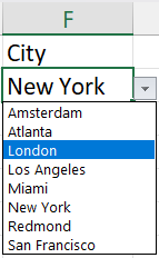
The dropdown itself draws from both data sources, ensuring users can only select valid cities. This list, generated in cell H1, demonstrates another level of data integration:
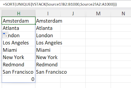
Notice how column B from Source 1 combines with column A from Source 2. The UNIQUE and SORT functions create a clean, alphabetized list. However, observe the "0" value in cell H9—this represents a data quality issue that appears when we have blank cells in our source data.
Cleaning the Dropdown with TOCOL
Column I presents the refined version, eliminating that problematic zero:
.png)
The enhanced formula incorporates the TOCOL function with parameter 1 to ignore blank cells:
=TOCOL(SORT(UNIQUE(VSTACK(Source1!B2:B,000, Source2!A2:A,000))),1)
This parameter ensures blank cells don't create unwanted entries in our dropdown—a crucial detail for maintaining data integrity in professional applications.
Implementing Data Validation
The final step connects our dynamic list to the dropdown through Excel's data validation feature:
.png)
The reference I1# utilizes Excel's spill range notation, automatically adjusting when our city list expands or contracts. This dynamic referencing ensures our dropdown remains current as underlying data changes—a hallmark of robust spreadsheet design.
This comprehensive approach to data integration showcases how modern Excel can handle complex data consolidation tasks that previously required specialized database tools or extensive VBA programming. The techniques demonstrated here are particularly valuable for financial analysts, data managers, and business intelligence professionals working with diverse data sources in Excel 365 environments.