Suppose cell A1 contains this formula:
=A2
Do you know what that means? Many Excel users think it means to pick up the data from Cell A2. If you're one of those users, you're not alone—and you're not entirely wrong. But what if cell C3 contained the same =A2 formula? Does it mean the same thing? Here's where most users get tripped up, and understanding the difference will transform how you work with spreadsheets.
Here's the truth: these users are partly right, but they're missing a crucial concept. What =A2 really means from cell A1 is "pick up the value from the cell which is one row below this one." What =A2 means from cell C3 is "pick up the value from the cell which is 1 row up and 2 columns to the left." Excel isn't thinking in absolute terms—it's thinking in relative positions.
This distinction between relative and absolute references is fundamental to Excel mastery, yet it's one of the most misunderstood concepts among users at all levels. Once you grasp this principle, you'll understand why formulas behave the way they do when copied, and you'll be able to build more sophisticated, flexible spreadsheets.
Let's test your understanding with a practical example.
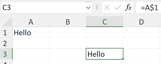
Suppose you have this spreadsheet:
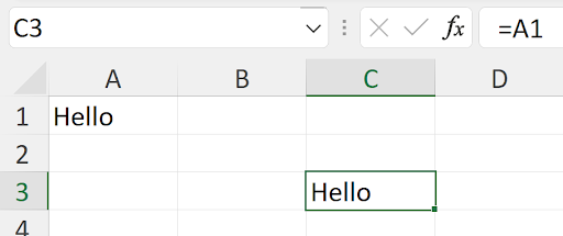
Now, here's the challenge: if you copy cell C3 and paste it into cell D3, what will you see? And what if you copy cell C3 and paste it to cell A2? Before you scroll down, take a moment to think through the relative positioning logic we just discussed.
In neither case will you see "Hello"—and that's the key insight. Pasting into cell D3 will give you 0, while pasting into cell A2 will give you the dreaded #REF! error. Here's what actually happens:
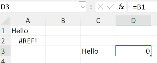
When you copied cell C3 and pasted to D3, what you actually copied was the instruction "go 2 rows up and 2 columns to the left." When Excel executes this instruction from D3, it lands on cell B1, which contains 0. When you paste the same instruction to cell A2, Excel tries to go 2 rows up from A2 (impossible—there's nothing above row 1) and 2 columns to the left of column A (also impossible). The result? Excel throws a #REF! error, indicating the reference doesn't exist.
This behavior explains why so many spreadsheet formulas break when users copy and paste without understanding relative references. The solution lies in Excel's absolute reference system.
Excel provides an elegant solution through absolute references, indicated by the "$" symbol. From Cell C3, a reference to cell A1 written as =$A$1 means exactly that: cell A1. No relative positioning, no left/up/right/down calculations. It means A1, period.
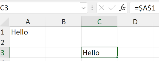
Now, copying cell C3 and pasting it anywhere will consistently return "Hello", since the pasted formula will always contain =$A$1. This is the foundation of reliable spreadsheet design—knowing when your references should move and when they shouldn't.
But Excel offers even more precision through mixed references, which combine relative and absolute positioning. These references use the "$" symbol selectively: =$A1 locks the column but allows the row to change, while =A$1 locks the row but allows the column to change. This granular control is invaluable for complex calculations and data models.
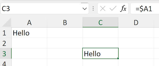
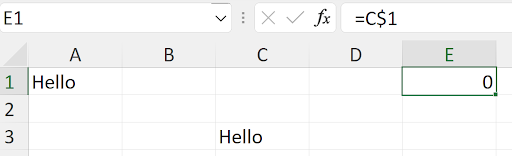
When you copy cell C3 to cell D4, observe how the mixed reference behaves:

Notice how moving one row down and one column right changed the row reference from 1 to 2, but the column reference remained locked at A. The "$" before the "A" held it in place while allowing the row number to adjust relatively.
The reverse works equally well:
Here, the mixed reference A$1 locks row 1 while maintaining the relative column positioning (2 columns to the left). When copying cell C3 to E1, watch how this plays out:
The reference to row 1 remained fixed, while the column reference maintained its relative position (2 columns to the left). This behavior is consistent whether you're filling right, down, or copying to any location—wherever there's a "$" in the reference, that component stays locked.
Let's apply these principles to solve a real-world problem: building a multiplication table that works correctly when copied.
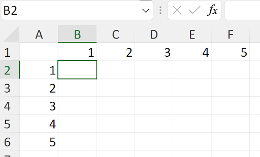
What formula should go into cell B2 so that when you fill it right to column F and then fill the entire range B2:F2 down to row 6, you get a proper multiplication table? This is where many users stumble, but the solution demonstrates the power of mixed references.
The naive approach—using =B1*A2 and filling right and down—creates this disaster:
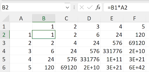
Why does this fail? Because each cell is multiplying the cell directly above by the cell directly to the left, creating a cascade of unintended calculations. In a proper multiplication table, you want each cell to multiply its column header (row 1) by its row header (column A). This requires strategic use of mixed references.
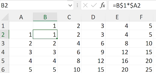
The correct formula =B$1*$A2 uses mixed references to lock the row reference for the column headers and the column reference for the row headers. Each cell locks onto the appropriate header values while allowing the other dimension to change as the formula is copied. Notice how cell D4 demonstrates this principle in action:

When you truly understand these reference types and can predict how they'll behave when copied, you've mastered one of Excel's most powerful features. This knowledge will help you build more robust financial models, data analysis tools, and automated calculations that work consistently across your entire spreadsheet. In 2026's data-driven business environment, this level of spreadsheet proficiency isn't just helpful—it's essential for professional credibility.