Pandas Overview
Pandas stands as one of the most powerful Python libraries for data manipulation and analysis, transforming raw, messy datasets into actionable insights. While the name might evoke images of adorable bears, "Pandas" actually derives from "Panel Data" — a term borrowed from econometrics that reflects its sophisticated analytical roots. In today's data-driven landscape, mastering Pandas operations has become essential for data scientists, analysts, and developers working with real-world datasets.
This comprehensive tutorial will guide you through five fundamental Pandas operations that form the backbone of effective data manipulation:
- Loading Dataframes
- Joining and Merging Dataframes
- Adding and Deleting Columns
- Deleting Null Values
- Analysis and Checking Data Types
Key Pandas Operations
Data Loading
Import CSV and Excel files into dataframes for analysis. Supports multiple file formats including JSON and TXT.
Data Joining
Merge dataframes using common columns. Essential for combining datasets from different sources.
Column Management
Add, delete, and rename columns dynamically. Create new features through column operations.
Pandas stands for Panel Data, a term borrowed from econometrics, not the animal despite the cute association.
Loading Dataframes
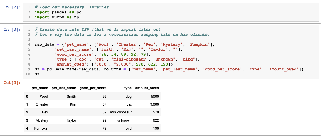
In professional data workflows, you'll primarily encounter data stored in CSV files or Excel spreadsheets. These formats remain the standard for data exchange across industries, making them your starting point for most analysis projects. Let's begin by creating a practical example using veterinary clinic data — a scenario that demonstrates common data challenges you'll face in real applications.
In this code, we've constructed a dataframe directly within Pandas, but real-world scenarios require converting this data into persistent file formats. The ".to_csv()" method serves this purpose, creating a comma-separated values file that can be shared, stored, and loaded across different systems and applications.
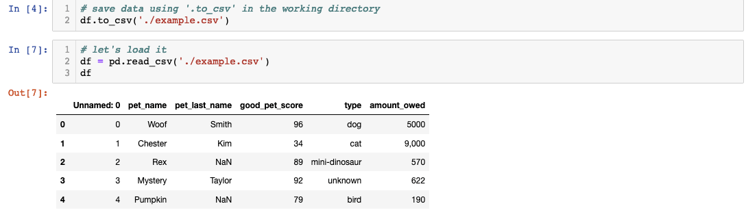 The first step involves saving your dataframe as a CSV file in your designated working directory. Note that directory paths will vary depending on your operating system and project structure — always verify your path before proceeding. Once saved, Pandas' ".read_csv()" method seamlessly transforms the file back into a working dataframe, ready for manipulation and analysis.
Excellent progress! However, data rarely exists in isolation. Imagine discovering additional information stored in a separate Excel file — in our case, a "bad behavior score" for each pet that provides crucial context for our analysis. This scenario mirrors real-world data challenges where information is distributed across multiple sources and formats.
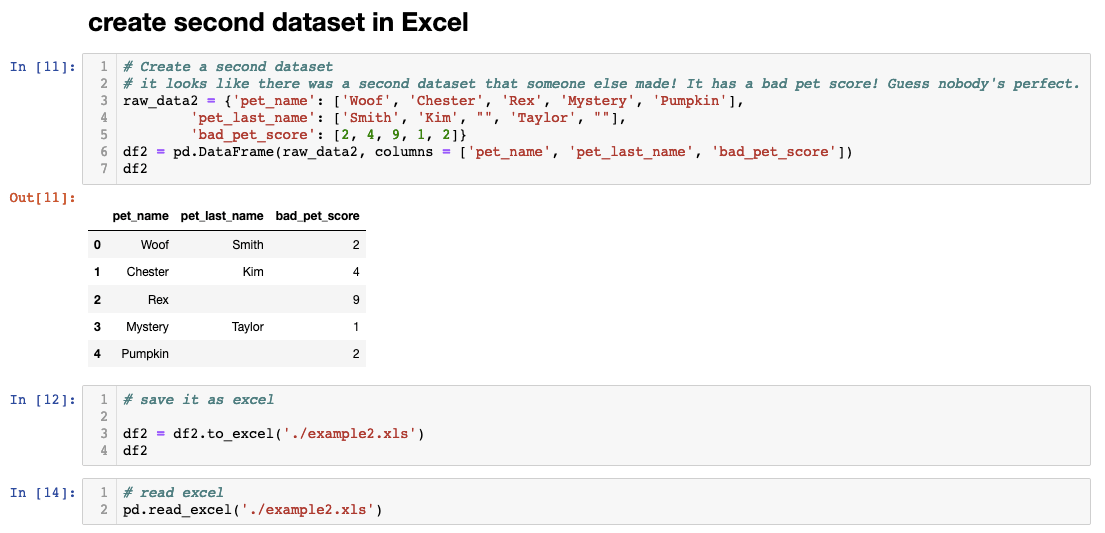
One of Pandas' greatest strengths lies in its ability to unify disparate data sources. Whether you're working with CSV files, Excel spreadsheets, JSON APIs, or plain text files, Pandas standardizes everything into a consistent dataframe format. This capability proves invaluable in enterprise environments where data often originates from multiple systems, databases, and third-party sources. Now that we have multiple dataframes representing different aspects of our data, let's explore how to combine them effectively.
Loading Data Process
Create Sample Data
Build a dataframe with veterinary client data including pet names and amounts owed
Export to CSV
Use the .to_csv() method to save the dataframe to your working directory
Read CSV Back
Import the CSV file using pandas .read_csv() method to create a new dataframe
Load Excel Files
Import additional data from Excel files containing supplementary information like bad scores
File Format Support
| Feature | CSV | Excel |
|---|---|---|
| Method | .read_csv() | .read_excel() |
| File Size | Smaller | Larger |
| Features | Simple | Multiple Sheets |
Joining and Merging Dataframes
Data integration represents one of the most critical skills in modern data analysis. When separate dataframes share common identifiers — like the pet names in our example — these columns become the foundation for combining datasets. This process, known as joining or merging, allows you to create comprehensive datasets from fragmented information sources.
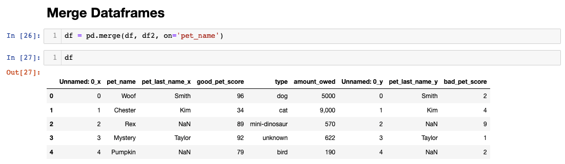
Notice how Pandas intelligently handles column name conflicts during the merge process. When duplicate column names exist across dataframes, Pandas automatically appends suffixes ("_x" and "_y") to distinguish between sources. This behavior prevents data loss while clearly indicating the origin of each column. The variable reassignment of "df" demonstrates a common practice in data workflows — iteratively building more complete datasets through successive operations.
Pandas offers multiple join types (inner, outer, left, right) that mirror SQL database operations, giving you precise control over how records are combined. Understanding these options becomes crucial when working with datasets of different sizes or when dealing with missing records across sources. With our merged dataset complete, let's address the inevitable cleanup tasks that follow data integration.
Adding and Deleting Columns
Data cleanup represents a significant portion of any analysis project — often consuming 60-80% of your time. Our merged dataset contains redundant columns (those with "_y" suffixes) and automatically generated index columns that clutter our workspace and potentially confuse downstream analysis.
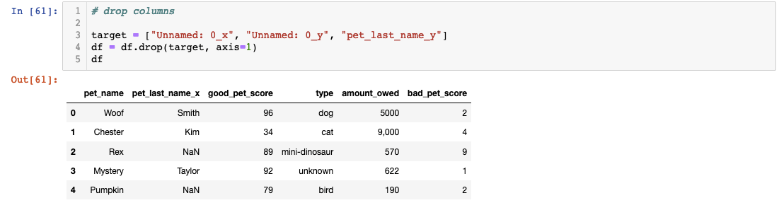
The drop operation removes unwanted columns efficiently, but pay attention to the column selection logic. Removing redundant merge artifacts and auto-generated indices keeps your dataset clean and interpretable — crucial factors when sharing your work with colleagues or stakeholders who need to understand your data structure quickly.
Column renaming addresses another common cleanup task: making column names more descriptive and consistent with your organization's naming conventions:
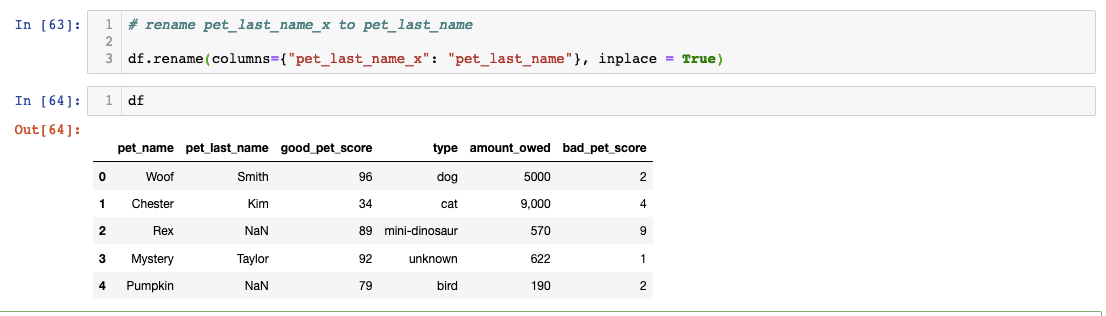
The "inplace=True" parameter deserves special attention. Without this flag, Pandas creates a new dataframe with your changes, leaving the original unchanged. While this behavior provides safety against accidental modifications, it can lead to confusion when changes don't appear to "stick." In production environments, consider whether you need to preserve original data states before applying inplace operations.
Beyond cleanup, column operations enable feature engineering — creating new variables that enhance your analysis. Let's demonstrate by calculating a composite score that combines positive and negative behavioral metrics:
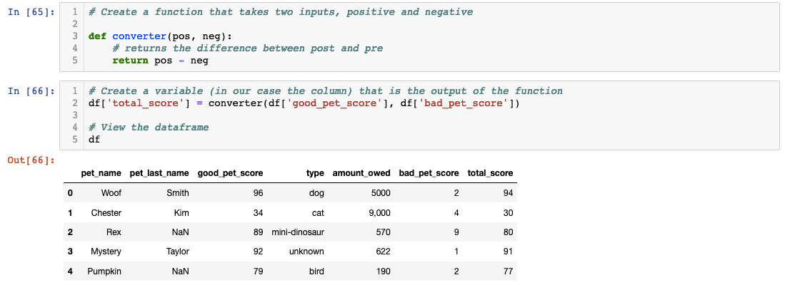
This approach showcases best practices for feature creation: define reusable functions for complex calculations, then apply them to create new columns. Feature engineering often determines the success of subsequent analysis, as well-constructed variables can reveal patterns invisible in raw data. This skill becomes particularly valuable in machine learning contexts where engineered features frequently outperform raw inputs.
Column Management Tasks
Remove columns automatically created with 'y' endings during merges
Delete 'Unnamed: 0' columns created automatically by Pandas
Use descriptive names that reflect the actual data content
Ensure modifications are saved to the dataframe permanently
Creating new columns based on existing data is called feature engineering - a fundamental data science technique.
Deleting Null Values
Missing data presents one of the most challenging aspects of real-world data analysis. Our dataset contains pets without last names, representing animals from shelter partnerships where different data collection standards apply. Rather than viewing missing data as a problem, consider it an opportunity to make informed business decisions about data inclusion criteria.
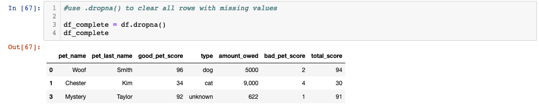
The decision to exclude pro bono cases from billing analysis makes business sense, but notice our approach: creating a new variable (df_complete) rather than overwriting the original dataset. This practice preserves data lineage and allows for alternative analysis approaches. In professional settings, you might need to analyze the complete dataset for operational insights while using the cleaned version for financial reporting.
Pandas offers sophisticated missing data handling beyond simple deletion, including forward-fill, backward-fill, and interpolation methods. The choice depends on your data's nature and analysis requirements. Always document your missing data decisions, as they significantly impact analysis validity and business conclusions.
Handling Missing Data
Create new variables for cleaned data instead of overwriting originals - you might need the complete dataset later.
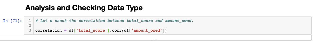
Analysis and Checking Data Types
With our dataset cleaned and prepared, we can now explore relationships within the data. Let's investigate whether pet behavior correlates with veterinary costs — a hypothesis with clear business implications for treatment planning and pricing strategies.
Pandas provides built-in statistical methods like ".corr()" for quick correlation analysis, but successful analysis depends on proper data types:
 The error message "unsupported operand type(s) for /: 'str' and 'int'" reveals a common data quality issue: numeric values stored as strings. This problem frequently occurs when importing data from external sources, especially spreadsheets where number formatting can introduce non-numeric characters like commas, currency symbols, or trailing spaces.
Data type verification should be standard practice before any quantitative analysis. Use the ".dtype" attribute to inspect column types and identify potential issues before they derail your analysis:
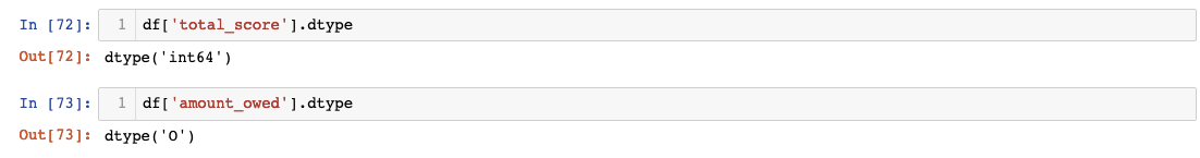
The "object" dtype often indicates string data or mixed types — a red flag for numeric analysis. Converting these columns requires careful preprocessing to remove formatting artifacts that prevent proper type conversion:
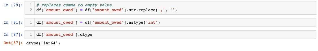
This two-step process — removing non-numeric characters, then converting data types — represents a fundamental pattern in data cleaning. Many real-world datasets require similar preprocessing to handle currency symbols, percentage signs, or regional number formatting differences.
With properly formatted data, we can now calculate our correlation: df['total_score'].corr(df['amount_owed']) returns -0.722088.
This strong negative correlation (-0.72) indicates that pets with lower behavioral scores tend to generate higher veterinary bills — confirming our hypothesis that problematic behaviors lead to increased medical interventions. In business terms, this insight could inform client communication strategies, preventive care programs, or risk assessment models for treatment planning.
While visualization tools like Seaborn and Matplotlib would enhance this analysis with compelling charts and graphs, the correlation coefficient alone provides actionable intelligence. This tutorial demonstrates how Pandas transforms raw data into business insights through systematic manipulation, cleaning, and analysis — skills that remain fundamental to data-driven decision making across all industries.
Data Type Correction Process
Identify the Problem
Check correlation and encounter data type errors between string and integer columns
Examine Data Types
Use .dtype to verify column data types - int64 for integers, 'O' for objects/strings
Clean String Data
Remove formatting characters like commas that prevent type conversion
Convert Data Types
Change column data types to appropriate formats for numerical analysis
Correlation Analysis Result
The -0.722088 correlation shows a strong negative relationship between total score and amount owed in the veterinary data.