Rearranging Data with New Functions in Excel

Rearranging Data with New Functions

Excel's modern array functions have revolutionized how we manipulate and reorganize data. In this comprehensive guide, we'll explore six powerful functions that will streamline your data transformation workflows: TOCOL, TOROW, WRAPCOLS, WRAPROWS, CHOOSECOLS, and CHOOSEROWS. These functions, part of Excel's dynamic array capabilities, eliminate the need for complex workarounds and manual copy-paste operations that once plagued spreadsheet users.

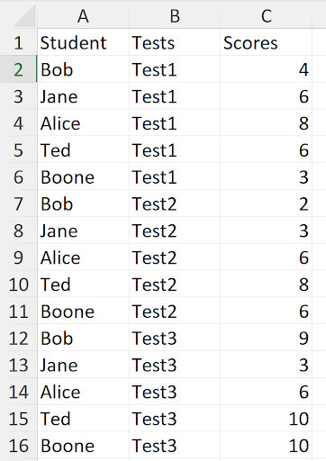
Let's begin with TOCOL, a function that transforms any array arrangement into a single vertical column. Consider this common scenario: you have test scores arranged in a grid format and need to convert them into a simple list for analysis or reporting.

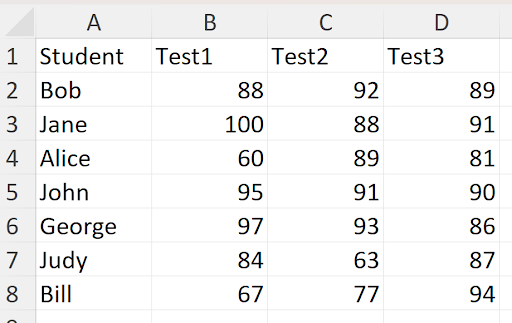
The TOCOL function excels at this transformation task. Its syntax follows a logical structure: =TOCOL(array, ignore, scan_by_column). The array parameter (B2:D8 in our example) defines your source data. The "ignore" parameter allows you to skip blank cells, errors, or both—crucial for maintaining clean datasets. The "scan_by_column" parameter controls the reading direction, which we'll examine shortly.

Here's the result:

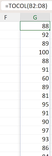
By default, TOCOL reads data horizontally first—notice how the values flow from Bob's test scores across row 2 (columns B, C, then D) before moving to row 3. This left-to-right, then top-to-bottom pattern mirrors how we naturally read text. However, you can reverse this behavior by setting the scan_by_column parameter to TRUE, making the function read vertically first:

This vertical-first approach groups all Test1 scores together before moving to Test2 scores in cell G8—a powerful feature for organizing data by categories or time periods.

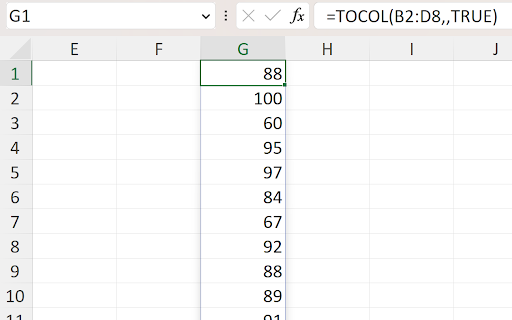
TOROW functions as TOCOL's horizontal counterpart, arranging array data into a single row rather than a column. This function proves invaluable when creating dashboard headers or preparing data for horizontal charts and visualizations:

While you could achieve similar results with =TRANSPOSE(TOCOL(B2:B8,, TRUE)), using TOROW directly creates cleaner, more readable formulas. In professional environments where formula maintenance matters, this clarity translates to reduced errors and easier troubleshooting.

Moving beyond simple flattening operations, let's explore CHOOSECOLS—a selective filtering function that extracts specific columns from your data arrays. Instead of manually copying columns or creating complex INDEX-MATCH combinations, CHOOSECOLS provides surgical precision for column selection. Suppose you need to display only names and Test3 scores from your original dataset:

CHOOSECOLS makes this extraction effortless:

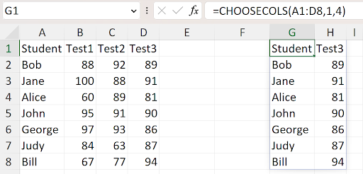
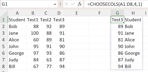
The function accepts the source array (A1:D8) followed by column numbers to display—in this case, columns 1 and 4. Beyond selection, CHOOSECOLS excels at reordering columns. Simply adjust the sequence of column numbers to rearrange your output:

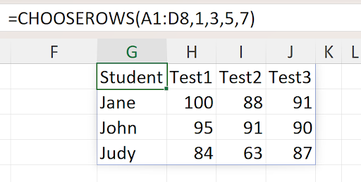
CHOOSEROWS operates with identical logic but targets rows instead of columns. This function shines when filtering data by categories, time periods, or specific criteria. For instance, to isolate students whose names begin with "J" while preserving the header row:

The real power emerges when combining these functions. To create a vertical list from the filtered "J-student" results, nest CHOOSEROWS within TOCOL:

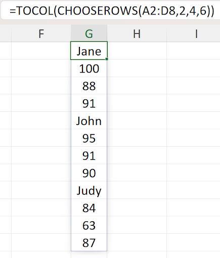
This formula first filters rows 2, 4, and 6 from range A2:D8, then flattens the results into a single column. Such function combinations create sophisticated data transformations that would previously require multiple steps or VBA programming.

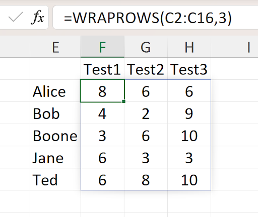
Now we shift focus to WRAPCOLS and WRAPROWS—functions that reverse the flattening operations of TOCOL and TOROW. These functions reshape linear data into multi-dimensional arrays, essential for creating formatted reports and structured layouts. Consider this vertical list of scores that needs reorganization:

Our goal is transforming this linear arrangement into a structured grid format:

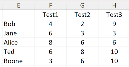
This transformation requires a strategic three-function approach. The formulas reside in cells F1, E2, and F2, each serving a specific purpose in the data restructuring process.

The formula in F1 creates the column headers:

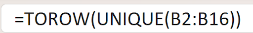
This formula nests UNIQUE within TOROW to extract distinct test names and arrange them horizontally. While =TRANSPOSE(UNIQUE(B2:B16)) would achieve the same result, using TOROW demonstrates modern Excel best practices and expands your functional toolkit for complex scenarios.

Cell E2 contains a straightforward label:

The crucial transformation occurs in F2 with the WRAPCOLS function:

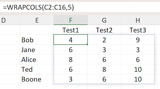
WRAPCOLS takes the vertical score list and wraps it into columns every 5 rows. Since each test contains exactly 5 scores, this parameter creates perfect alignment—when the function reaches the third score in F6, it automatically wraps to column G for Test2 scores.

Data organization often varies, requiring different wrapping strategies. Consider this alternative arrangement where data is grouped by student rather than test:

When data clusters into 3-item groups (student names followed by their three test scores), WRAPROWS becomes the appropriate tool for restructuring in cell F2:

WRAPROWS creates new rows every 3 columns, perfectly aligning with our student-centric data structure. This flexibility between WRAPCOLS and WRAPROWS ensures you can handle virtually any linear-to-grid transformation requirement in your professional work.